LLM AB Tests

There’s been a good bit of discussion about synthetic surveys (here and here). It’s an interesting time because LLMs are adding new capabilities to get all sorts of information that you couldn’t have before. But simultaneously it seems that most of that information is bullshit in the Frankfurtian sense. What are we to do?

As statisticians, I think we are uniquely suited to this problem. Careful titration of information and representations of uncertainty are our superpowers. So if anyone is going to responsibly take account of these new tools it might as well be us.

This fits nicely with AB testing. Tests are expensive both in time and opportunity cost of showing the worse variant. You might be tempted to run your LLM and let it tell you that A is better than B. Surely that’s some sort of prior information about B being better than A? Of course prior is maybe the wrong word here. I really don’t have a clue what the relationship is between the LLM verdict and outcome. So really it’s more like a data synthesis problem. I have some data from the LLM telling me about the conclusion of interest and some data from the AB test telling me about the same thing. Let’s combine them in a principled manner.

The Data

For concreteness, let’s consider the Upworthy Research Archive (Matias et al., 2021¹), a public dataset of 32487 A/B experiments run by Upworthy between 2013 and 2015. Each row is one headline+image variant (a “package”) with columns for impressions and clicks (CTR is clicks / impressions). We use the exploratory subset (4873 tests, 22666 packages), downloaded from the Open Science Framework.

We only have access to the headlines now; the images are just saved by ids. Ideally you could have sent both to a multimodal LLM², but for now we’ll only consider the 2515 headline pairs which share the same images.

I’ll be using the Gemini API to obtain my verdicts. This was the final outcome after a painful odyssey of trying open source models. Note that open source performance was roughly similar to what you see below: it was just super slow. I was suprised to find that I wasn’t charged for this but their billing information is confusing so confidence is low.

import json
import os
import sys
import time
from typing import Literal

import pandas as pd
from google import genai
from pydantic import BaseModel, Field

MODEL = "gemini-3.1-flash-lite"

class Verdict(BaseModel):
    analysis: str = Field(description="Brief analysis of both headlines considering emotional appeal, curiosity gap, specificity, and clarity.")
    verdict: Literal["A", "B"] = Field(description="Which headline will get more clicks: A or B.")


COMPLETED_STATES = {
    "JOB_STATE_SUCCEEDED",
    "JOB_STATE_FAILED",
    "JOB_STATE_CANCELLED",
    "JOB_STATE_EXPIRED",
}

def prompt(ha: str, hb: str) -> str:
    return (
        "You are judging which of two news article headlines is more likely to be clicked.\n\n"
        f'Headline A: "{ha}"\n'
        f'Headline B: "{hb}"\n\n'
        "First, briefly analyse the two headlines: consider emotional appeal, curiosity gap, "
        "specificity, and clarity. Then give your verdict returning exactly 'A' or 'B'."
    )


def build_request(ha: str, hb: str) -> dict:
    return {
        "contents": [{"role": "user", "parts": [{"text": prompt(ha, hb)}]}],
        "config": {
            "response_mime_type": "application/json",
            "response_schema": Verdict,
            "temperature": 0,
        },
    }


def poll_until_done(client, job_name: str) -> object:
    job = client.batches.get(name=job_name)
    while job.state.name not in COMPLETED_STATES:
        print(f"  state: {job.state.name} — sleeping 30s…")
        time.sleep(30)
        job = client.batches.get(name=job_name)
    return job


def main():
    outfile = "data/processed/filtered-data-with-verdicts.csv"
    if os.path.isfile(outfile):
        print(f"File {outfile} already exists")
        return

    api_key = os.environ.get("GEMINI_API_KEY")
    if not api_key:
        print("Error: GEMINI_API_KEY environment variable not set")
        sys.exit(1)

    client = genai.Client(api_key=api_key)
    df = pd.read_csv("data/processed/filtered-data.csv")

    requests = [build_request(row.headline_a, row.headline_b) for row in df.itertuples()]
    print(f"Submitting batch of {len(requests)} requests…")

    job = client.batches.create(
        model=MODEL, src=requests, config={"display_name": "ab-headlines"},
    )
    print(f"Created job: {job.name}")
    job = poll_until_done(client, job.name)
    print(f"Job finished: {job.state.name}")

    if job.state.name != "JOB_STATE_SUCCEEDED":
        print(f"Error: {getattr(job, 'error', 'unknown')}")
        sys.exit(1)

    responses = job.dest.inlined_responses
    raw_file = outfile.replace(".csv", "-raw.jsonl")
    with open(raw_file, "w") as f:
        for row, r in zip(df.itertuples(), responses):
            f.write(json.dumps({
                "headline_a": row.headline_a, "headline_b": row.headline_b,
                "text": r.response.text if r.response else None,
                "error": str(r.error) if r.error else None,
            }) + "\n")

    rows, errors = [], 0
    for row, r in zip(df.itertuples(), responses):
        key = f"{row.headline_a!r} vs {row.headline_b!r}"
        if r.error:
            print(f"  error ({key}): {r.error}")
            rows.append({"headline_a": row.headline_a, "headline_b": row.headline_b, "verdict": "missing", "analysis": None})
            errors += 1
        else:
            try:
                parsed = Verdict.model_validate_json(r.response.text)
                rows.append({"headline_a": row.headline_a, "headline_b": row.headline_b, "verdict": parsed.verdict, "analysis": parsed.analysis})
            except Exception as e:
                print(f"  parse error ({key}): {e} — raw: {r.response.text!r}")
                rows.append({"headline_a": row.headline_a, "headline_b": row.headline_b, "verdict": "missing", "analysis": None})
                errors += 1

    pd.DataFrame(rows).to_csv(outfile, index=False)
    print(f"Wrote {len(rows)} rows ({errors} errors) to {outfile}")


if __name__ == "__main__":
    main()

And performance is, uh, not great. We can check by computing the t-score for each pair and plotting its distribution split by verdict. If the model has any signal the two distributions should be shifted apart:

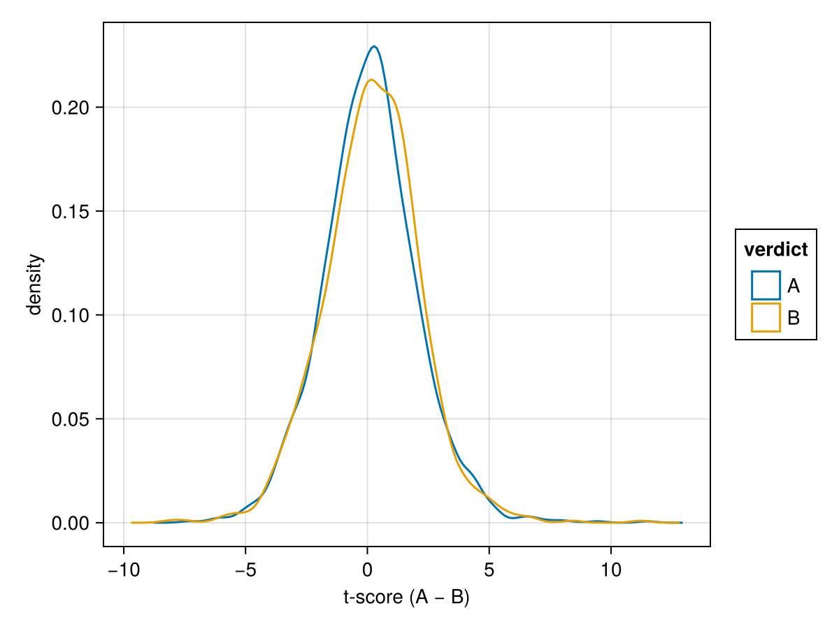
In some respects this is probably the best case for this blog post: if it were really accurate, you’d just go for the LLM verdict and forget all this trouble about AB tests. You can maybe get more mileage out of a better prompt or model, so we’ll also simulate an actually useful model.

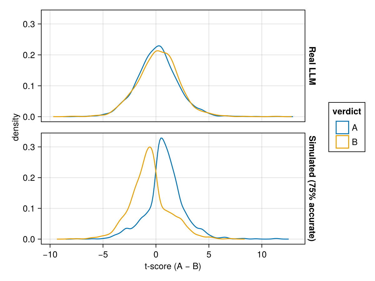
Much better separation than the LLM. Now let’s build the machinery to make use of whatever signal we do have.

Model

A nice Bayesian model for our AB test has two latent parameters \(p_{A,t}\) and \(p_{B,t}\) representing the CTR probability of each headline for this trial. We have

\begin{align*} p_{A,t} &\sim \mathrm{Beta}(\alpha, \beta) \\ p_{B,t} &\sim \mathrm{Beta}(\alpha, \beta) \\ c_{A,t} &\sim \mathrm{Binomial}(n_{A,t},\, p_{A,t}) \\ c_{B,t} &\sim \mathrm{Binomial}(n_{B,t},\, p_{B,t}) \end{align*}

where \(c_{*,t}\) stands for clicks.

Our LLM verdict is clearly trying to provide information on \(p_{A,t} > p_{B,t}\) so let’s just introduce that as an indicator function. But crucially we don’t believe it fully: so we think it’s only correct with probability ρ. We’ll have the latent state \(z_{t}\) represent whether our LLM is correct or incorrect on this trial.

\begin{align*} \rho &\sim \mathrm{Beta}(\kappa, \kappa) \\ z_t &\sim \mathrm{Bernoulli}(\rho) \\ v_t &= z_t\,\mathbb{1}[p_{A,t} > p_{B,t}] + (1-z_t)\,\mathbb{1}[p_{A,t} < p_{B,t}] \end{align*}

Note that \(\rho\) is shared across all of our trials. Let’s talk about that later.

Actually making it run

N.B. this section gets in the weeds of sampling: great for students or Bayesian inference nerds; the rest can skip to the results.

This is a rather hard geometry to sample from: we have a very sharp discontinuity at \(p_{A} = p_{B}\) for every single test! We’ll need to be really careful to make sure that our model is converging. Indeed, just running the model as is we observed R-hat \(\approx 1.7\) and ESS \(\approx 12\) in practice (on a reduced sample even), confirming the sampler couldn’t explore the space.

using Turing
@model function naive_rho_model(verdicts, ca, na, cb, nb)
    ρ ~ Beta(5, 5)
    p_a ~ filldist(Beta(2, 100), length(verdicts))
    p_b ~ filldist(Beta(2, 100), length(verdicts))
    for i in eachindex(verdicts)
        ca[i] ~ Binomial(na[i], p_a[i])
        cb[i] ~ Binomial(nb[i], p_b[i])
        lp = verdicts[i] == 1 ?
            log(p_a[i] > p_b[i] ? ρ : 1.0 - ρ) :
            log(p_b[i] > p_a[i] ? ρ : 1.0 - ρ)
        Turing.@addlogprob! lp
    end
end

The fix is to marginalize out \(p_{A,t}\) and \(p_{B,t}\) analytically. So we have the full posterior

\begin{align*} p(p_{A,t}, p_{B,t}, z_t, \rho \mid c_{A,t}, c_{B,t}, v_t) &\propto p(\rho) \prod_t \Bigl[ p(z_t \mid \rho)\, p(p_{A,t})\, p(c_{A,t} \mid p_{A,t})\, p(p_{B,t})\, p(c_{B,t} \mid p_{B,t})\, p(v_t \mid p_{A,t}, p_{B,t}, z_t) \Bigr] \end{align*}

We can then integrate out \(p_{A,t}\) and \(p_{B,t}\) together, and since the joint factorizes over the tests \(t\) the integral reduces to a product of per-test integrals:

\begin{align*} p(z_t, \rho \mid c_{A,t}, c_{B,t}, v_t) &\propto p(\rho) \prod_t p(z_t \mid \rho) \nonumber\\ &\quad \times \int_0^1\!\int_0^1 p(p_{A,t})\, p(c_{A,t} \mid p_{A,t})\, p(p_{B,t})\, p(c_{B,t} \mid p_{B,t})\, p(v_t \mid p_{A,t}, p_{B,t}, z_t)\; dp_{A,t}\, dp_{B,t} \end{align*}

The per-test integral has a nice structure. Start with the click terms: Beta priors and Binomial likelihoods are conjugate, so

\begin{align*} p(p_{A,t})\, p(c_{A,t} \mid p_{A,t}) &= \frac{p_{A,t}^{\alpha-1}(1-p_{A,t})^{\beta-1}}{B(\alpha,\beta)}\, \binom{n_{A,t}}{c_{A,t}} p_{A,t}^{c_{A,t}}(1-p_{A,t})^{n_{A,t}-c_{A,t}} \nonumber\\ &= m_{A,t}\cdot\mathrm{Beta}(p_{A,t};\,\tilde\alpha_{A,t},\,\tilde\beta_{A,t}) \end{align*}

where \(\tilde\alpha_{A,t} = \alpha + c_{A,t}\), \(\tilde\beta_{A,t} = \beta + n_{A,t} - c_{A,t}\), and \(m_{A,t} = \binom{n_{A,t}}{c_{A,t}}\frac{B(\tilde\alpha_{A,t},\,\tilde\beta_{A,t})}{B(\alpha,\beta)}\) is the Beta-Binomial marginal likelihood (a constant in \(p_{A,t}\)). The same holds for the B arm with \(m_{B,t}\).

Now for the verdict. The likelihood \(p(v_t \mid p_{A,t}, p_{B,t}, z_t)\) is a hard indicator: if \(v_t = A\), it equals \(\mathbb{1}[p_{A,t} > p_{B,t}]\) when \(z_t = 1\) (LLM correct) and \(\mathbb{1}[p_{A,t} < p_{B,t}]\) when \(z_t = 0\) (LLM wrong). So for fixed \(z_t\) the double integral reduces to integrating a product of two independent Beta densities over half the unit square:

\begin{align*} I_t(z_t = 1,\, v_t = A) &= m_{A,t} m_{B,t} \int_0^1\!\int_0^1 \mathrm{Beta}(p_A;\,\tilde\alpha_{A,t},\,\tilde\beta_{A,t})\, \mathrm{Beta}(p_B;\,\tilde\alpha_{B,t},\,\tilde\beta_{B,t})\, \mathbb{1}[p_A > p_B]\; dp_A\, dp_B \nonumber\\ &= m_{A,t} m_{B,t}\, q_t \end{align*}

where \(q_t = P(X_A > X_B)\) with \(X_A \sim \mathrm{Beta}(\tilde\alpha_{A,t}, \tilde\beta_{A,t})\) and \(X_B \sim \mathrm{Beta}(\tilde\alpha_{B,t}, \tilde\beta_{B,t})\) drawn independently. Math Stack Exchange doesn’t think there is a closed form for this probability in general, but it is cheap to estimate by Monte Carlo. By symmetry note that \(I_t(z_t = 0,\, v_t = A) = m_{A,t} m_{B,t}\,(1-q_t)\).

With the integral in hand, summing out our binary \(z_t\) to complete the marginalization is just two terms:

\begin{align*} \sum_{z_t \in \{0,1\}} p(z_t \mid \rho)\, I_t(z_t) &= \rho\cdot m_{A,t} m_{B,t}\, q_t + (1-\rho)\cdot m_{A,t} m_{B,t}\,(1-q_t) \nonumber\\ &= m_{A,t} m_{B,t}\,\bigl[\rho\, q_t + (1-\rho)(1-q_t)\bigr] \end{align*}

The \(m_{A,t} m_{B,t}\) factors are constants in \(\rho\) and drop out of the posterior. Handling \(v_t = B\) symmetrically (which swaps \(q_t\) and \(1-q_t\)), the full marginal posterior for \(\rho\) is

\[p(\rho \mid \mathbf{v}, \mathbf{c}) \propto p(\rho) \prod_t \begin{cases} \rho\, q_t + (1-\rho)(1-q_t) & v_t = A \\ (1-\rho)\, q_t + \rho\,(1-q_t) & v_t = B \end{cases}\]

This is a smooth function of \(\rho\) alone without discontinuities or latent variables. We end up with a clean 1D model that NUTS samples trivially (ESS \(\approx 4000\), R-hat \(= 1.000\)).

using Statistics, Random

const ALPHA, BETA = 2, 100  # Beta(2, 100) prior: mean CTR ≈ 2%

function prob_a_gt_b(ca, na, cb, nb; α=ALPHA, β=BETA, S=50_000)
    mean(rand(Beta(α+ca, β+na-ca), S) .> rand(Beta(α+cb, β+nb-cb), S))
end
ab_df.q = [prob_a_gt_b(r.clicks_a, r.impressions_a, r.clicks_b, r.impressions_b)
            for r in eachrow(ab_df)]

@model function rho_model(verdicts, q)
    ρ ~ Beta(5, 5)
    for i in eachindex(verdicts)
        p = verdicts[i] == 1 ? q[i]*ρ + (1-q[i])*(1-ρ) :
                               q[i]*(1-ρ) + (1-q[i])*ρ
        Turing.@addlogprob! log(p)
    end
end

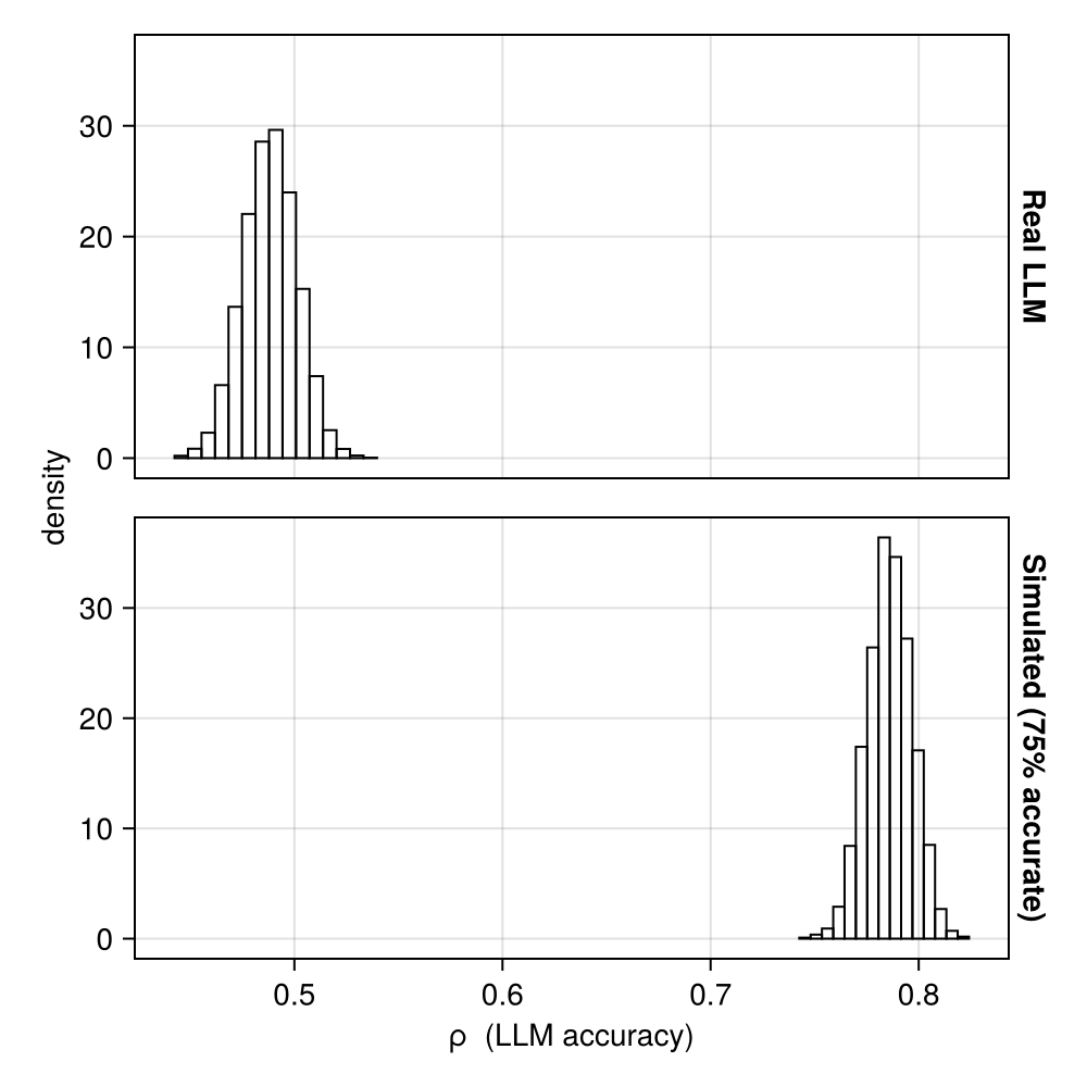
Results

We can first check that it works: the posteriors for \(\rho\) cluster pretty tightly around the real agreement values (the simulated verdicts by chance ended up a little high).

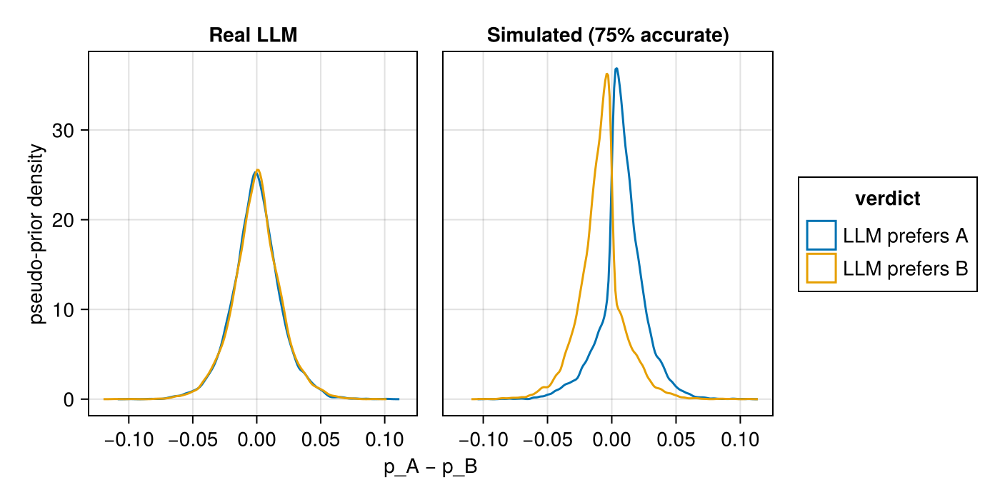
We can visualize the information that we provide as a sort of pseudo-prior (technically it’s the posterior from the other data). Before seeing any data aside from the real LLM verdict, we can see the following posteriors for positives and negatives: basically it’s not strong enough to overcome the actual evidence. The simulated verdicts, on the other hand, gives us some strong information.

As we start collecting more data we consider the posterior predictive distribution for a new AB test with counts \(c_{A,t*}\), \(n_{A,t*}\), \(c_{B,t*}\), \(n_{B,t*}\). We have

\[p(p_{A,t^*}, p_{B,t^*} \mid c_{A,t^*}, c_{B,t^*}, v_{t^*}, \hat\rho) \propto \mathrm{Beta}(p_{A,t^*};\,\tilde\alpha_{A,t^*},\tilde\beta_{A,t^*})\, \mathrm{Beta}(p_{B,t^*};\,\tilde\alpha_{B,t^*},\tilde\beta_{B,t^*})\, \ell_{t^*}(\hat\rho)\]

where \(\hat\rho\) is plugged in from the posterior (or we can average over it). As we collect more data we fall into three cases:

1. Clear agreement: the AB data and LLM verdict point the same way
2. Weak conflict: the AB test is inconclusive, so the LLM shifts the posterior noticeably
3. Strong conflict: the AB data and LLM verdict disagree

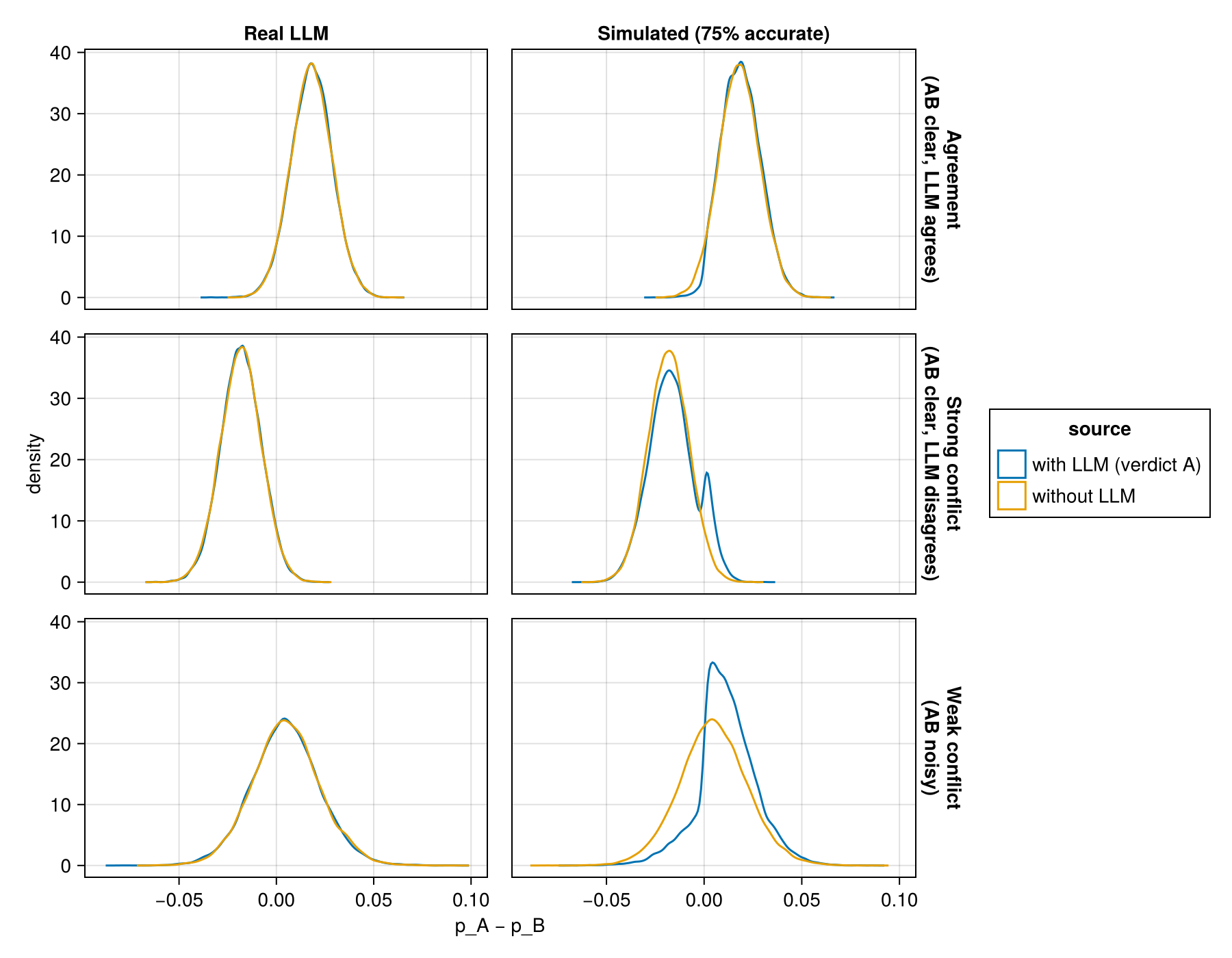
And indeed we find that the real LLM correctly gives us no information: this is exactly what we wanted. However once you have helpful verdicts this changes: the agreement case doesn’t particularly change things as you would expect. But the conflict cases you see strong effects pushing the weak conflict case strongly towards the LLM verdict. This can be overcome however as more AB observations come in but still gives you a little bimodality right at zero due to the LLM verdict boost.

Where do we go from here?

The simplest thing is just to try to find even better models or prompts. This has the effect of driving \(\rho\) higher and, justifiably, giving more weight to the LLM verdict. That said, I’m not entirely sure this is possible, at least for this task. I’d rather view this process as providing a safety harness for enabling further experimentation in this space. Most cynically, you can feel free to let your engineers AI their brains out, and so long as you keep it within this model framework there’s limited harm they can do.

The one harm, though, is that they could overfit to the historical data which would drive \(\rho\) up artificially. There’s a deeper philosophical question though: why should there be any connection at all between historical AB tests and the LLM verdicts? This comes down to a judgment call: if you think it holds you believe this model; otherwise you don’t and should discard it. For instance, we wouldn’t expect this same \(\rho\) to hold for, say, Economist articles: the audience and purpose are just too different. We’re making an assumption about the stationarity and homogeneity of our headline distributions with this shared \(\rho\).

Statistically trying to improve this model becomes hairy: this is definitely a toy problem. In reality AB tests are useful for measuring many different result metrics and the nice clean conjugacy breaks pretty quickly. We also don’t necessarily care about just the absolute difference in metrics: in the face of multiple metrics the relative differences are important so you can make tradeoffs. And we don’t always care about just two alternatives: you’re probably running 3+ headlines. You could decompose this into 1v1 tests, but I’m not sure your LLM will respect transitivity.

Thus, I just want to point to this as an example of how we might use LLMs: not as ground truth, but as a semi-reliable source of side information. With principled statistical models we can get the benefits without the costs.